
Download Our Excel Functions Template Below
Inventory control formulas in Excel can increase the efficiency and productivity of your business as you become more organized in your inventory management. As your business grows, you need to keep up with the growing demands, and Microsoft Excel can help you do that.
20 Useful Microsoft Excel Formulas for Inventory Management
Basic inventory management is easier with inventory management Excel formulas. The program offers a host of options and shortcuts that aren’t necessarily intuitive, so here are 20 you should know when choosing an Excel spreadsheet for your inventory management.
1. SUM: =SUM(VALUE:VALUE)
The SUM function works to add values through individual values, cell references, cell ranges or a combination of the three of them. This will often look like adding the values of a row or column. If this is the case, a shortcut is to select the last cell in the row or column and hit Alt+.
2. SUMIF: =SUMIF(RANGE,CRITERIA,[sum_range])
The SUMIF formula builds on the SUM formula but allows you to specify the criteria you are looking to get the sum of. The range specifies the range of cells you want to be evaluated by the criteria, which should be in the form of a number, expression, reference text or function. This helps distinguish the sum of the value of products for a specific customer or something similar.
3. SUMPRODUCT =SUMPRODUCT(RANGE1,RANGE2)/SELECT CELL
Another variation of the SUM formula, SUMPRODUCT allows you to add, subtract, multiply or divide products from a certain range. Multiplication is the default operation, but to change it, you simply replace the commas with the operator you want. This helps calculate shipment and return values or sales averages by various markers.
4. Incoming Stock: =SUMIF(INCOMINGS[PRODUCT CODE]; [@[PRODUCT CODE]];INCOMINGS[QUANTITY])
You can use Excel to count your incoming stock using a variation of the SUMIF function combined with your product codes. This will help when it comes time for an inventory audit as there will be fewer discrepancies between the numbers in your channels and the physical amount of inventory you have. You can lower stress and the amount of work you have to do in the long run as this function can help you manage your stock levels appropriately.
5. Outgoing Stock: =SUMPRODUCT(($B5=item)*(movtype="Outgoing")*(quantity))
The outgoing stock formula works with the SUMPRODUCT function to help you easily calculate how much inventory has been sold and shipped. This formula can help you keep better, more accurate data and avoid overselling.
6. Stock Level: =[@[INITIAL STOCK]]+[@INCOMINGS]=[@OUTGOINGS]
Excel can combine the formulas you have already into a new formula so you can see what your current stock level is based on the incomings and outgoings. This is helpful when looking into ordering more inventory, as you will quickly be able to see how much you have in stock. However, this only works if you constantly update your ingoing and outgoing stock formulas so you know those are correct at any given time.
7. FIND or LOOKUP: =FIND(TEXT,WITHIN_TEXT, [START_NUMBER]) or =SEARCH(TEXT,WITHIN_TEXT, [START_NUMBER])
Being able to find data quickly in all your values is extremely useful. Mastering this formula can increase your efficiency greatly. The FIND function allows you to isolate small, specific data, while the LOOKUP function allows you to perform a wider search.
8. VLOOKUP: =VLOOKUP(LOOKUP_VALUE,TABLE_ARRAY,COL_UNDEX_NUM, [RANGE_LOOKUP])
The VLOOKUP function is helpful in situations when you need to find things in a table or a range in a row. Using it, you can combine data you’ve located with another value. If you want to find the total value of an order, linking it to the various products it contains, using the VLOOKUP function can make that happen.
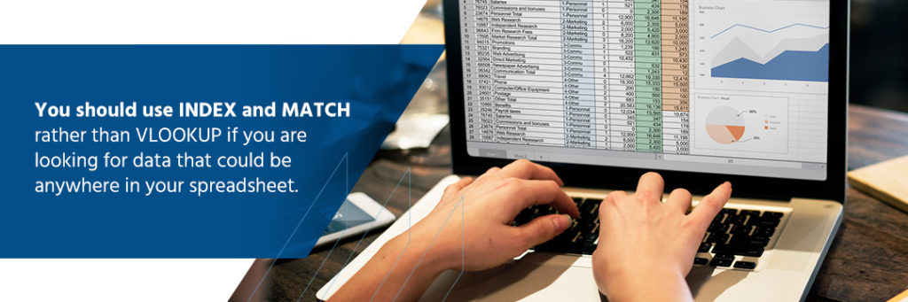
9. INDEX and MATCH: =INDEX(Profit column,MATCH(Lookup Value,Product Name column,0))
The INDEX function allows you to return a value to a value within a table. It fills in the gap left by the VLOOKUP formula in its ability to read only left to right. The MATCH function searches for an item within a given range of cells before giving you the relative position of the value you are searching for.
You should use these functions rather than VLOOKUP if you are looking for data that could be anywhere in your spreadsheet.
10. LEFT or RIGHT: =LEFT(SELECT CELL,NUMBER); =RIGHT(SELECT CELL,NUMBER)
Using these functions allows you to move quickly from the beginning and end of the cell. Naturally, the LEFT function returns you to the first, or first several, characters in a cell, while the RIGHT function jumps you to the last, or last several, characters in a cell.
11. RANK: =RANK(SELECT CELL, RANGE_TO_RANK_AGAINST, [ORDER])
The RANK function allows you to order values in a numbered list based on their value relative to each other. You can choose to arrange them in ascending or descending order. This is helpful when you want to tangibly see which products are selling most or least, what has the highest stock value or which product you need to order the most of.
12. AVERAGEIF: =AVERAGEIF(SELECT CELL, CRITERIA, [AVERAGE_RANGE])
This function gives you the arithmetic mean, or the average, of the cells in the range you specify. The formula is similar to the RANK formula but gives you a unique value that can help you monitor how your business changes over time.
13. CONCATENATE: =CONCATENATE(SELECT CELLS YOU WANT TO COMBINE)
The CONCATENATE function allows you to combine data, whether that’s numbers, text, dates or other values. It is most commonly used to join text together but is very helpful for creating stock-keeping units (SKU).
14. LEN: =LEN(SELECT CELL)
The LEN function allows you to determine the number of characters in a text string in a designated cell. If you use Excel to keep track of your product codes, this is a helpful way to identify them quickly.
15. COUNTA: =COUNTA(SELECT CELL)
The COUNTA function lets you count the cells that are not empty within a certain range. This allows you to identify data omission, an issue that is necessary to identify in product omission.
16. COUNTIF: =COUNTIF(range, "criteria")
This formula is a more specific version of the COUNTA function. The COUNTIF function allows you to build clearer criteria for what values you want to be counted. This can give you better data in various areas of your spreadsheet.
17. TRIM: =TRIM("text")
The TRIM function removes spaces from the text you select, aside from single spaces between words. This allows you to clean up your text and get rid of excess spacing. When searching for terms later, this can prevent some data from not showing up simply because of a spacing issue.
18. VALUE: =VALUE("text")
With this helpful function, you can replace text that represents a value with the value itself in number form. You can designate the format to change in other ways as well.
19. DAYS: =DAYS(SELECT CELL, SELECT CELL)
The DAYS function allows you to determine the number of days that occurred between two dates in your data. When looking at inventory and attempting to determine when to order different products, this function can save you a lot of time.
20. MINIF and MAXIF: =MINIFS(RANGE1, CRITERIA1, RANGE2); =MAXIFS(RANGE1, CRITERIA1, RANGE2)
These Excel formulas can help you find inventory data more quickly. The MINIFS function provides you with the minimum value that exists within a designated range of cells. You can quickly see your lowest number of products sold or lowest price. The MAXIF function does the same thing with the maximum value.

Learning the best Excel formulas for inventory management can increase your efficiency and productivity in a small way. Finale Inventory can take that and build on it, providing you with world-class service and the best cloud inventory software for your business.
Excel Formulas for Inventory Management FAQ
What Excel formula is used for inventory?
There is no single inventory formula. Common Excel formulas for inventory include SUM for totals, SUMIF or SUMIFS for condition-based totals, SUMPRODUCT for value calculations, and a basic stock formula such as Beginning Inventory + Incoming Stock – Outgoing Stock = Current Stock.
How to use Excel for inventory management?
Excel can be used for inventory management by creating a spreadsheet with columns like item name, SKU, quantity on hand, unit cost, supplier, reorder level, and location. Formulas, filters, conditional formatting, and lookup functions can then be used to track stock levels, flag low inventory, and organize product data.
What are the 7 basic Excel formulas?
Seven basic Excel formulas often used as a starting point are SUM, AVERAGE, COUNT, MIN, MAX, IF, and VLOOKUP.
Does Excel have an inventory template?
Yes, Excel includes inventory templates that can be used to track products, quantities, costs, and stock movement. These templates can be customized to fit different inventory needs.
How to create an inventory spreadsheet?
To create an inventory spreadsheet, start with columns such as SKU, item name, description, quantity, unit cost, supplier, reorder point, and location. Then add formulas to calculate totals and stock levels, apply filters to make sorting easier, and use conditional formatting to highlight low-stock items.
